bibliography@authorIndex
LaTeX and all its little helpers are your friends … most of the time. However, every once in a while they decide to do some nasty stuff and annoy you.
The Quest for the Lost @
Imagine you’re preparing a citation in BibTeX where the author is an institution called author = {iSleep@Work} (@s seem to be very trendy in names nowadays). Using natbib and the *.bib-file in your document, you run latex/bibtex and everything works.
Later you decide to include an index of authors in your appendix, add all the code to your document (\usepackage{makeidx}\citeindextrue\makeindex in the preamble and \printindex in the appendix), but suddenly latex yells that there’s something wrong …
Looking at the document, you will see that all citations in the body are correct and also the references-section has not changed. The problem lies in the author index section, where the entry for your citation now reads Work – something happened to the iSleep@.
BibTeX vs. MakeIndex
Contrary to BibTeX, MakeIndex uses the @ internally. An index reference called sortByThis@displayThis will only read ‘displayThis’, but will be sorted by sortByThis – so we see that the @ and everything before is skipped. That’s what happened to the iSleep@! The MakeIndex manual suggests that the @ will be displayed if we insert a double quote before it, yet this also shows up in all the BibTeX entries, so it’s not an option.
How to fix it …
The solution is embarrassingly simple: just replace the @ (at least in your author tags that will be used by makeindex) with \char"0040{} in your *.bib-file and everything should work (the example above now is author = {iSleep\char"0040{}Work}).
Explanation: we can avoid the @ sign by inserting it as a unicode character by number, so makeindex does not interpret it as the `sorting’ command and prints the field properly.
Poor man’s thumb indices in LaTeX
Custom Thumb Indices
I’m currently writing my diploma thesis in LaTeX and if you devote yourself (along with a lot of time) to this task, you want it to look good (or at least I do).
One of these days I figured, “I want a thumb index in by thesis”, so I started looking for some easy solution. I found the package thumb that, together with fancyhdr, can be used to generate thumb indices. It worked, but one problem was that my painstakingly adjusted KOMA-Script headers and footers vanished and besides I wanted a more “custom” look than just some bars at the edges of my pages. I also came across a bulk of code for thumb indices (within KOMA) that wouldn’t work for me either.
Some time ago I made a DIN A0 poster in LaTeX. I remembered that I used a background image then, so I dug up some code and re-discovered the package wallpaper.
I admit that this solution is not perfect as it requires manual work and adjustment (i.e. constructing the indices for every chapter), but aesthetically it definitely pays off because you don’t have consider any restrictions in terms of design.
The workflow is basically like this:
(0) Determine how many chapters your report/book will have.
(1) Design the backgrounds for each chapter.
(2) Integrate the designed pages as backgrounds for each chapter.
(3) Marvel at your beautiful custom thumb indices, or start again at (1).
Example: Four Chapters w/appendix
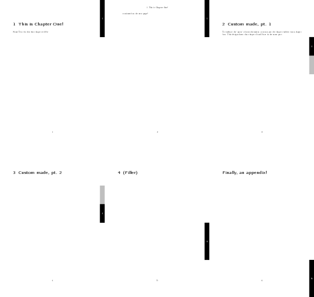
(1) For the example I chose simple black boxes containing chapters’ numbers. If you have some parts in your book that you want to `tie together’ visually, you can also use a larger container in another color for the range of the part (here chapters 2 and 3). One big advantage of this approach is that you are not restricted to LaTeX to design the background, but can use tools like InkScape for example (although I used pstricks here).
Attention: Design your backgrounds a little larger than the final page to avoid annoying gaps at the edges of your page (even a few millimeters will do the trick).
(2) To include the backgrounds, two commands are used right after each chapter:
\ClearWallPaper — deletes any previous background images
\TileWallPaper{width}{height}{image} — includes the image on this and subsequent pages unless \ClearWallPaper is used. Attention! use the width and height of the (larger) background image.
LaTeX-Code
\documentclass[USenglish,fontsize=12pt,
paper=a4,oneside,pdftex,version=last]{scrbook}

\usepackage[T1]{fontenc}
\usepackage[ansinew]{inputenc}
\usepackage{xcolor,graphicx,wallpaper}

\begin{document}
\mainmatter
\chapter{This is Chapter One!}
\ClearWallPaper\TileWallPaper{220mm}{297.4mm}{thumb_1.pdf}
Some Text for this first chapter will be\ldots
\newpage
\ldots continued on the next page!

\chapter{Custom made, pt. 1}
\ClearWallPaper\TileWallPaper{220mm}{297.4mm}{thumb_2.pdf}
To indicate the `parts' of your document, you can put the chapter indices into
a larger box. This design shows that chapter 2 and 3 are in the same part.

\chapter{Custom made, pt. 2}
\ClearWallPaper\TileWallPaper{220mm}{297.4mm}{thumb_3.pdf}

\chapter{(Filler)}\ClearWallPaper\TileWallPaper{220mm}{297.4mm}{thumb_4.pdf}

\backmatter
\chapter{Finally, an appendix!}
\ClearWallPaper\TileWallPaper{220mm}{297.4mm}{thumb_A.pdf}

\end{document}
Run pdflatex and that’s it! As you can see, the code can only be used for one-sided documents, but it shouldn’t be too difficult to work out a way to switch between wallpapers on odd and even pages.
The source code along with the thumb index backgrounds can be downloaded here: Custom Thumbs Indices – Source and the compiled version should look like this: Custom Thumb Indices (PDF).
Getting data in and out of R (Part 4)
Myth 3b: You can’t get data from R into Excel.
You guessed it – getting data from R into Excel works just as easy the other way round via the clipboard (see the previous post). It’s not (yet) possible to select and copy all data from an object in the spreadsheet view, but that’s no problem because there are other convenient solutions.
As we’ve used read.table() to read the clipboard’s contents, we can use the function write.table() and copy data into it. For the sake of compactness I will just give an example for matrices, because it works the same for vectors.
Let’s generate some random data first
> set.seed(1) > x = data.frame(a=rnorm(10),b=rnorm(10),c=rnorm(10),d=letters[1:10]) > xa b c d 1 1.35867955 -0.1645236 0.3981059 a 2 -0.10278773 -0.2533617 -0.6120264 b 3 0.38767161 0.6969634 0.3411197 c 4 -0.05380504 0.5566632 -1.1293631 d 5 -1.37705956 -0.6887557 1.4330237 e 6 -0.41499456 -0.7074952 1.9803999 f 7 -0.39428995 0.3645820 -0.3672215 g 8 -0.05931340 0.7685329 -1.0441346 h 9 1.10002537 -0.1123462 0.5697196 i 10 0.76317575 0.8811077 -0.1350546 j
When we look at the help for write.table() we see a lot of parameters to tweak:
write.table(x, file = "", append = FALSE, quote = TRUE, sep = " ",
            eol = "\n", na = "NA", dec = ".", row.names = TRUE,
            col.names = TRUE, qmethod = c("escape", "double"))
The parameter file is set to an empty string ("") by default what tells R to print the output in the console. This is great to try new parameters because you don’t have to paste something to Excel to see the results, so I will not write to "clipboard" for the moment.
> write.table(x,file="")"a" "b" "c" "d" "1" 1.35867955152904 -0.164523596253587 0.398105880367068 "a" [ . . . output omitted . . . ] "10" 0.763175748457544 0.881107726454215 -0.135054603880824 "j"
Looks good, but wait … the header contains four variables while there are five columns of data! The parameter row.names = TRUE is responsible for this, chances are that you don’t need this vector because there’s some other ID-variable in your data, so let’s drop it.
> write.table(x,file="",row.names=FALSE)"a" "b" "c" "d" 1.35867955152904 -0.164523596253587 0.398105880367068 "a" [ . . . output omitted . . . ] 0.763175748457544 0.881107726454215 -0.135054603880824 "j"
Now the number of columns in the header and data match, but Excel will still not be able to read it, because the delimiter is set to " ". We need to change this parameter to tab using sep="\t".
> write.table(x,file="",row.names=FALSE,sep = "\t")"a" "b" "c" "d" 1.35867955152904 -0.164523596253587 0.398105880367068 "a" [ . . . output omitted . . . ] 0.763175748457544 0.881107726454215 -0.135054603880824 "j"
At this point we could already send the data to the clipboard (file="clipboard") and paste it into Excel without problems, but for the sake of completeness I will show some other parameters that you might need as well.
If you have missing values these will be copied as "NA" and Excel can’t interpret it, so set na="" to leave these cells empty. If you don’t want to copy variable names you can use col.names=FALSE. Usually you also don’t need strings to be quoted – quote=FALSE. And last but certainly not least some of you will need to change the decimal sign from point to comma dec=",".
Writing your own I/O functions
One seeming restriction of this approach might be the rather long command you need to enter in order to set all parameters the right way, e.g. write.table(x, file="clipboard", row.names=FALSE, sep = "\t", na="", quote=FALSE).
To remedy this just write your own function:
toExcel = function(x,varnames=TRUE){
   write.table(x, file="clipboard", row.names=varnames,
               sep = "\t", na="", quote=FALSE)
}
Now you have a nice little function and eliminated the problem of forgetting or messing up parameters when entering this looooong command.
It’s also a good idea to do something similar for the import function from my previous post:
fromExcel = function(varnames=TRUE){
   read.table("clipboard", header=varnames, sep = "\t")
}
Note that both functions have an argument (varnames=TRUE) to switch reading/writing of variable names on and off.
The only problem that remains is that you’d have to enter the definition of toExcel() and fromExcel() in every R session manually. To make both available in every started R session, open the file Rprofile.site in the /etc/ folder of your R distribution and append the functions’ definitions at the end. Now restart R and have fun with it.
Getting data in and out of R (Part 3)
Myth 3a: You can’t get data from Excel into R easily.
Nope. Although R can read data from all kinds of files (txt, csv, xls, dta, sav, …), there’s a quick way of transferring your from Excel to R.
Caveat: I haven’t tested how this works for other operating systems and/or spreadsheet programs – I have used Windows XP and Excel 2003 for all examples presented below.
Vectors
Method A
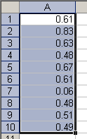
Getting a column of data into R is no big deal. Select what you want, copy it and enter data.object = scan(). Instead of entering single values as we did in the previous post, just paste the copied contents and submit a blank line to terminate scan():
Copy a vector in Excel
> data.object = scan() 1: 0.61 2: 0.83 3: 0.63 4: 0.48 5: 0.67 6: 0.61 7: 0.06 8: 0.48 9: 0.51 10: 0.49 11:Read 10 items> data.object[1] 0.61 0.83 0.63 0.48 0.67 0.61 0.06 0.48 0.51 0.49
If you have strings to read, remember specifying scan(what="character") (see part 2).
Method B
Instead of scanning all values, you can directly read the clipboard’s contents like this:
> data.clipb = readClipboard() > data.clipb[1] "0.61" "0.83" "0.63" "0.48" "0.67" "0.61" "0.06" "0.48" "0.51" "0.49"
Important: note that the created object will be character, so you have to convert the object to numeric.
> class(data.clipb)[1] "character"> data.clipb = as.numeric(data.clipb)
Matrices
To read matrices from Excel, you need the read.table() function (for help and options see ?read.table). You don’t have to pay attention to data types because R creates a data.frame and assigns suitable types to each column (i.e. variable).
Without Variable Names
Copying data from Excel without variable names
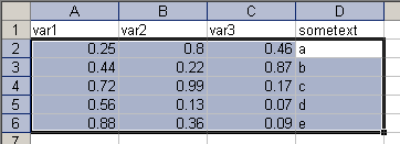
By default, read.table() has the option header=FALSE, this means that the first row is not interpreted as variable names, so I only select and copy the values of three numeric and one string variable. Now create a new object and assign read.table(file="clipboard") to it.
> data.noheader = read.table( + file="clipboard") > data.noheaderV1 V2 V3 V4 1 0.25 0.80 0.46 a 2 0.44 0.22 0.87 b 3 0.72 0.99 0.17 c 4 0.56 0.13 0.07 d 5 0.88 0.36 0.09 e
We see that the data were read successfully. To check the view internal structure of the data frame, type
> str(data.noheader)'data.frame': 5 obs. of 4 variables: $ V1: num 0.25 0.44 0.72 0.56 0.88 $ V2: num 0.8 0.22 0.99 0.13 0.36 $ V3: num 0.46 0.87 0.17 0.07 0.09 $ V4: Factor w/ 5 levels "a","b","c","d",..: 1 2 3 4 5
From this we see that our data frame has four variables with five observations. Three variables are numeric and for the string variable, a factor with five levels was created.
With Variable Names
Copying data with variable names
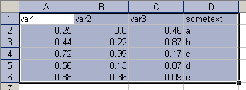
If you have variable names in the first row of your data set, you just have to add the option header=TRUE:
> data.header = read.table( + file="clipboard",header=TRUE) > data.headervar1 var2 var3 sometext 1 0.25 0.80 0.46 a 2 0.44 0.22 0.87 b 3 0.72 0.99 0.17 c 4 0.56 0.13 0.07 d 5 0.88 0.36 0.09 e
Problems with decimals
One problem I have not covered up to this point is the usage of other delimiters and decimal point characters. For instance, if you live in Germany, your operating system will most likely interpret decimal characters as a comma. So if you had problems using the scan() and read.table() function this may be the reason. To circumvent related problems, both functions have an option dec that is dec="." by default. Adjust this setting to whatever character you use as a decimal point and it should work fine.
> comma.values = scan(dec=",") 1: 1,1 2: 2,2 3: 3,3 4: 4,4 5:Read 4 items> comma.values[1] 1.1 2.2 3.3 4.4
Problems with delimiters
read.table() assumes that columns are separated by a tabulator – and that’s fine for Windows because copied matrices will have this format, but if you need another delimiter (e.g. comma, semicolon or a blank) use the option sep=",". I copied this to my clipboard in plain text:
1;2;3;4
5;6;7;8
9;9;9;9
Specifying the delimiters in R gives you the correct results
> read.table("clipboard",sep=";")V1 V2 V3 V4 1 1 2 3 4 2 5 6 7 8 3 9 9 9 9
Getting data in and out of R (Part 2)
In this post I want to continue where I left off last time. I showed the fix() and edit() functions to view and edit data frames. “But what about vectors” you might ask …
Myth 2: Inputting and editing vectors in R is tedious!
Everyone working with R is familiar with the c() function that combines its arguments into a vector. If you have to enter a vector manually you might do it this way:
> vec = c(1,2,3,4,10,20,30,40,100,200,300,400)
If this were the only way to create vectors it would really be annoying (imagine more data and decimal values – mix up some dots and commas and your vector’ll be a mess), but we can use a function called scan() that is more convenient for manually inputting vectors.
Basically it works like this: (1) Create a new object that will contain the data and assign scan() to it. (2) Enter your data hitting ‘enter’ after each datum. (3) When you are finished, submit a blank line (i.e. hit ‘enter’ once more) and R tells you how many items were read and assigned to the new object.
> vec.scan = scan() 1: 1 2: 2 3: 3 4: 4 5: 10 6: 20 7: 30 8: 40 9: 100 10: 200 11: 300 12: 700 13:Read 12 items

Edit a vector using the fix() or edit() functions.
I obviously made type error – element 12 should be ‘400’. I could use indices to correct this cell (vec.scan[12] = 400) or fix() (resp. edit(), see Getting data in and out of R – Part 1) which provides a more intuitive way of editing. Typing fix(vec.scan) opens a window where I can replace 700 with 400. Close it and you’re done.
What about characters?
No problem, scan() is a very versatile function (as we will see in subsequent posts) that can handle the data types logical, integer, numeric, complex, character, raw and list (see ?scan). So if you want to enter strings manually this could look like this:
> text.scan = scan(what="character") 1: scan() 2: can 3: read 4: text 5: and 6: also 7: special 8: characters 9: \/+-#$§%&_@ 10:Read 9 items> text.scan[1] "scan()" "can" "read" "text" "and" [6] "also" "special" "characters" "\\/+-#$§%&_@"
Note that you don’t have to quote text and additionally R escapes special characters as the backslash!
Beware of blanks!
By default R breaks up elements separated by blanks.
> scan(what="character") 1: this will not be one element 7:Read 6 items [1] "this" "will" "not" "be" "one" "element"
You can see that although there’s only one line of text, each word becomes a separate element. If you want each line to be a single element you can tell scan() to separate the input by another character, like the “new line” escape sequence:
> scan(what="character",sep="\n") 1: this is one element! 2:Read 1 item [1] "this is one element!"
The line was read as one element now.
Getting data in and out of R (Part 1)
I guess one major thing that scares people away from R (and makes them turn to ‘fluffy’ packages like SPSS etc.) is the seeming lack of the familiar spreadsheet user interface.
A couple of persons told me that they have trouble getting their data into SPSS, so they think they’d never be able to do it in R.
I have to disagree with them and below is a small list of I/O-related myths about R that need to be busted.
Myth 1: There are no spreadsheets in R!
No, there is a way to view your data in spreadsheet format and you can even input/edit your data using the same view.
Let’s generate a data frame containing seven variables with five (random) observations:
> set.seed(55)
> d = data.frame(v1 = rnorm(5), v2 = rnorm(5), v3 = rnorm(5), v4 = rnorm(5),
                 v5 = rnorm(5), v6 = rnorm(5), v7 = rnorm(5))
If we print this object, we get something like:
> dv1 v2 v3 v4 v5 v6 1 0.120139084 1.1885185 -0.04891095 -0.3662780 -1.5192720 0.960344 2 -1.812376850 -0.5053439 -0.84323377 2.3553639 1.4971178 -0.692181 3 0.151582984 -0.0992344 -2.07527077 1.0933772 0.8196153 1.405998 4 -1.119221005 0.3053532 -0.36076315 0.2858410 1.0660504 -1.633539 5 0.001908206 0.1984097 -0.63768966 0.9936578 0.7337559 0.261831 v7 1 1.5647544 2 0.3145893 3 -0.9346850 4 -0.1251366 5 -0.5267137
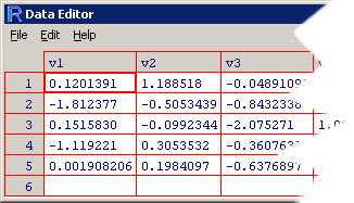 This kind of display is cumbersome because the set is split across variables (and we just have five observations and seven variables!). To destroy the first myth, use the
 edit() function on the data frame and you will see your data in a neat spreadsheet.
> edit(d)
But R can do a lot more. Suppose you want to enter some data manually. Create a new object and assign an empty data frame to it.
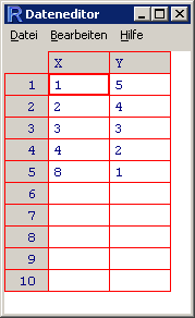 > dat.man = edit(data.frame())
The spreadsheet appears and you can change the variable names by clicking on them. I typed in the following data and viewed them again in R:
> dat.manX Y 1 1 5 2 2 4 3 3 3 4 4 2 5 8 1
If you spot a mistake in your data input, you’d have to assign the correct value to that cell. In larger sets it can be annoying to get the indices right, so you can use the edit() function to do this ‘graphically’.
dat.man = edit(dat.man) opens the editor again and you can go to the cell and edit the value. Note that you have to assign the edit() function’s result to an object. By using the fix() function you don’t have to reassign the edited data to the original object, so these two commands do the same:
> dat.man = edit(dat.man)
> fix(dat.man)Quick Tables with LaTeX
Today two friends of mine came for a visit and one of them mentioned LaTeX – he had to prepare a large table the other day and was quite annoyed. Setting tables in LaTeX can – even for seasoned users – be a daunting task. When I started out using LaTeX I had to face this fact early and I was very eager to find something to help me typeset tables quickly.
The Excel2LaTeX Plugin is a very effective utility to convert Excel sheets to LaTeX tables. You can download it from the CTAN (Comprehensive TeX Archive Network) here: http://tug.ctan.org/tex-archive/support/excel2latex/. After you have added it in Excel, an additional button will show up in your toolbar.
Using it is quite intuitive: highlight the cells you need in your table, click on the button (if some error message pops up, close it) and a new window with LaTeX code appears. The converter will also handle multicolumn cells, alignment and escape special characters ($, %, ^, …).
Putting on LaTeX …
As you can see I have switched from the nice but common layout to this darker theme. I also set up some links you might find interesting.
The main topic of this post is about the inclusion of (La)TeX in HTML. To keep the promises I’ve made in my mission statement, nice formulae will play an important role in this blog, so I was looking for a solution to this problem.
I found some code that was supposed to generate images using a server but that didn’t work very well. I’m kind of a DIY-guy, so I set up this minimalistic piece of code that generates a dvi-file and converts it into a png-image.
This is the LaTeX file:
\documentclass{article}
\pagestyle{empty} % clipping won't work with headers/footers
\begin{document}
$f(x|\mu,\sigma^2)=
\frac{1}{\sigma\sqrt{2\pi}}
\exp\left[-\frac{(x-\mu)^2}{2\sigma^2}\right]$
\end{document}
And to compile it type:
latex NameOfYourFile.tex
dvipng NameOfYourFile.dvi -D 100 -T tight
The optional -T tight clips off all borders around the formula (that’s why it is important to set \pagestyle{empty}).
You can adjust the image’s size by altering the resolution (the png below was created using -D 200) if something should be illegible (fractions!).

The Normal Distribution's probability density function (PDF) rendered in LaTeX
On the right you can see the result of the above code (not really: I manually inverted the colors).
I must admit that this approach isn’t very efficient if you need a lot of formulae, but if you only occasionally want to impress people visiting your site with a little math this might be worth a try.
First things first …
Yesterday I kind of happened to get my own domain and a friend of mine asked me to start a blog. Despite some initial doubts, the idea somehow grew on me so eventually I set this up and the first post is a mission statement in a way.
I’m not a big fan of blogs that extensively tell you what the blogger had for lunch or similar things, so one of my aims is to keep this place “chatter-free” (i.e. devoid of private stuff) except something remarkable happened (like when i finally finish my thesis!).
The rest of the posts will mainly revolve around psychology, science, statistics, programming, books, music and related topics. If I should stumble upon something interesting I would place it here, e.g. these days, I’m pretty much busy with the theory and practice of Bayesian data analysis.
Due to my lack of experience in blogging I cannot predict how (ir)regularly I will update this blog. However, if I’m not too short of time this is going to be a quite nerdy adventure I’m embarking on – and everyone who doesn’t think LaTeX is needed to produce shiny and tight clothes is invited to join me. 😉